Automatic processing of the seismic data is not practicable in some scenarios, e.g. slidequake monitoring on landslides, because sought after signals inNanoseismic Monitoring have such a low-SNR and are often only detected at single mini-arrays. Furthermore, comprehensive training of an automatic detector would be difficult because the occurrence of seismic signals can be infrequent and signal patterns can vary significantly depending on origin of the event. Automatic picking algorithms would either miss crucial events (false negatives) or create an abundance of events coming from the various noise sources.
Manual processing on the other hand allows an experienced seismologist with a deep knowledge of the setting and noise sources of the given area to set potential events into a broader context and thus eliminate false positives while finding even events disturbed by noise bursts. The need for manual screening of continuous data encouraged the development of a new software suite which is capable of displaying large datasets on the screen while preserving the capability to detect very weak and short lasting events. The usually used seismograms (time-domain) were not sufficient anymore and instead energies of seismic data are visualized in form of spectrograms (time-frequency domain). The spectrograms are enhanced by multiple signal processing steps and are called sonograms.
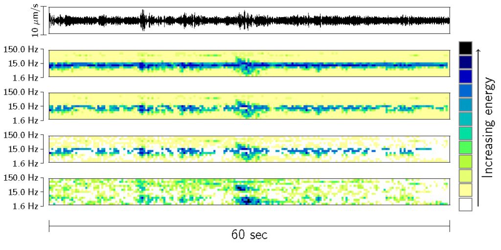
The above figure illustrates the processing steps of sonogram calculation for a local earthquake in a noisy environment. From top to bottom: seismogram, power spectral density spec-trogram with logarithmic amplitudes and half-octave frequency bands, noise adaptation, blanking and prewhitening. ML = 1.0 in 7.7 km distance).
The next step is to combine the calculated sonograms of each seismometer of a SNS to so-called Super-Sonograms.